Sagan and asymmetric risk

I watched a video recently of Carl Sagan discussing defense spending in contrast to spending on climate change prevention. His salient point is that if we used a small nonzero chance of annihilation to justify massive cold war spending in preparation for that possibility, we should be willing to do the same for mitigating climate change. This made me think about a natural comparison of the two which would guide climate spending:

P(x) C_x = I_x
P(y) C_y = I_y

Where x indicates the cold war, so C_x is the cost of the cold war occurring (with varying levels of calamity), and if we allow P(x) and C_x to be distributions we can sum or integrate over them to get the expected investment I_x to prevent them from occurring. We can do the same thing with climate change y, assuming C_y to be similarly ruinous (or even 10 or 20% as ruinous) and get the expected investment I_y to mitigate the risk. Obviously, the simplicity of this linear equation allows us to tweak the numbers to match our current understanding of the problems and associated risk, and everything just scales linearly. So if we think P(y)=1/2 P(x) and C_y=1/2 C_x, we should still have spent about a quarter of what we spent on the cold war on climate change mitigation.

Sagan’s point is clear and concise. The problem arises in our inability to grasp the nonlocal and nebulous future aspects of climate change, especially in places that haven’t yet been consistently negatively impacted (or have sufficient technology and energy to insulate from those effects via air conditioning , etc). But I also think that, even if we could understand the dangers associated with climate change, we would struggle with assessing the risks because they are asymmetric in time and effect.

Truly asymmetric or long-tail risks exist so far outside the normal distribution that it becomes challenging to intuit their likelihood and impact. The model we use to compare these (right side above) is a mixed regime of normal (gray) with long-tail skewed (red): X ~ (1-p) Nominal + p Tail. Nominal is the normal distribution and represents frequent/expected benign outcomes, while Tail is the heavy-tailed distribution of risks, and p is a rare event probability.

Some caveats worth calling out: here we’re using p to represent a discrete catastrophic event, like a Russian invasion or nuclear apocalypse in cold war terms or an extinction- or civilizational-event in climate change terms. The relative use of “rare” with respect to the cold war catastrophe can be used because of our understanding of the bomber gap and Russian doctrinal response to mutually assured destruction. I think it’s justified for use with respect to climate change because of the varied climates of earth mean the planet will almost certainly be able to support life somewhere, and the eventual obviousness of climate change will cause humanity to change course. It’s clear that the likelihood of “climate change events” is not p<<0.1 , it’s more like p=1. But p is in the eye of the beholder.

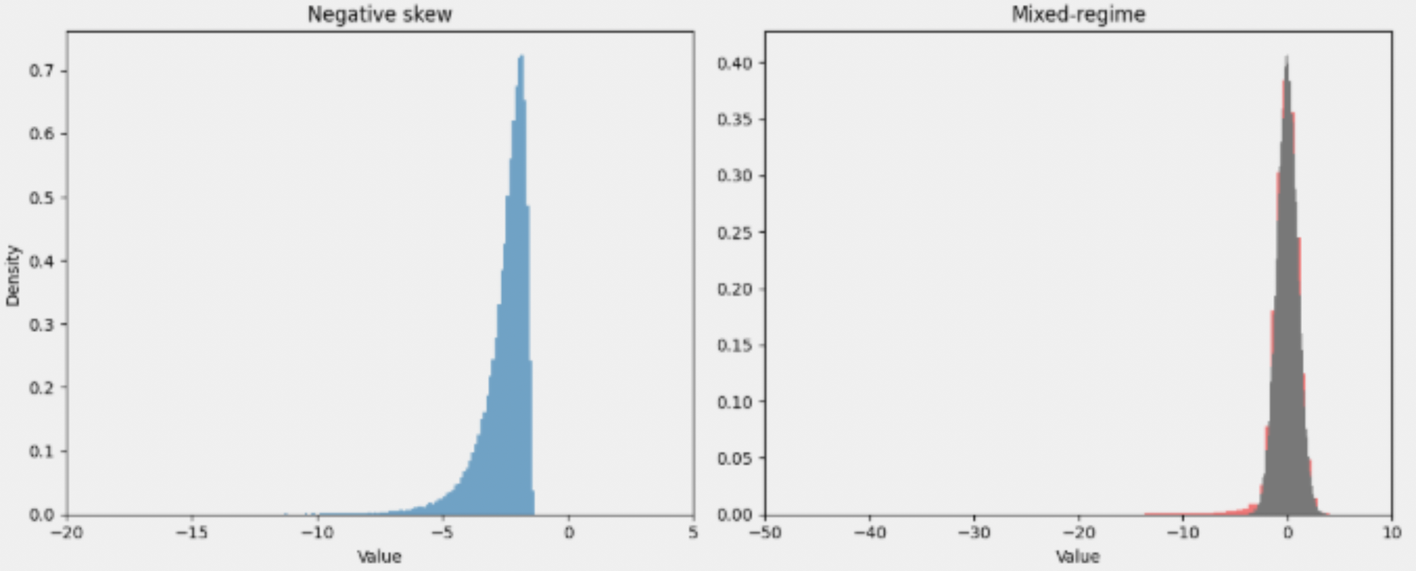
Our mixed regime combines normal N(mu, sigma^2) and Pareto distributions P(X<-x) ~ x^a . Using this, we can compare value at risk (VaR) and conditional VaR:

VaR(a) = inf{x : P(X <= x) >= a}
CVaR(a) = E[X | X <= VaR(a)]

In our example distributions, the failure mode (farthest left, located at -3.0 units) represented in the normal distribution had a VaR of -2.324 and CVaR of -2.663; the probability mass below -3.0 was 0.00136. In contrast, for the mixed regime with long negative tail, VaR and CVaR were -2.754 (comparable) and -5.957 (almost double), with 0.00756 of the probability mass below -3.0 (six times more mass).

The intuition of the CVaR (or CFaR for failure) is “how bad is bad?” In the normal case, there’s ~ 0.1% of a chance to have a failure, and that is increased to ~ 0.8% under the long-tail case. That’s a relative increase of about 6x, as I said above, but that’s not where the damage gets done. After all, we could have expanded the variance of the normal distribution to put 0.8% of the mass below -3.0 easily. The difference is that doing so would not significantly change the CVaR, which show impacts twice as large for the long-tail case. This makes the risk calculus much more complex since failure events are ruinous, not just bad.

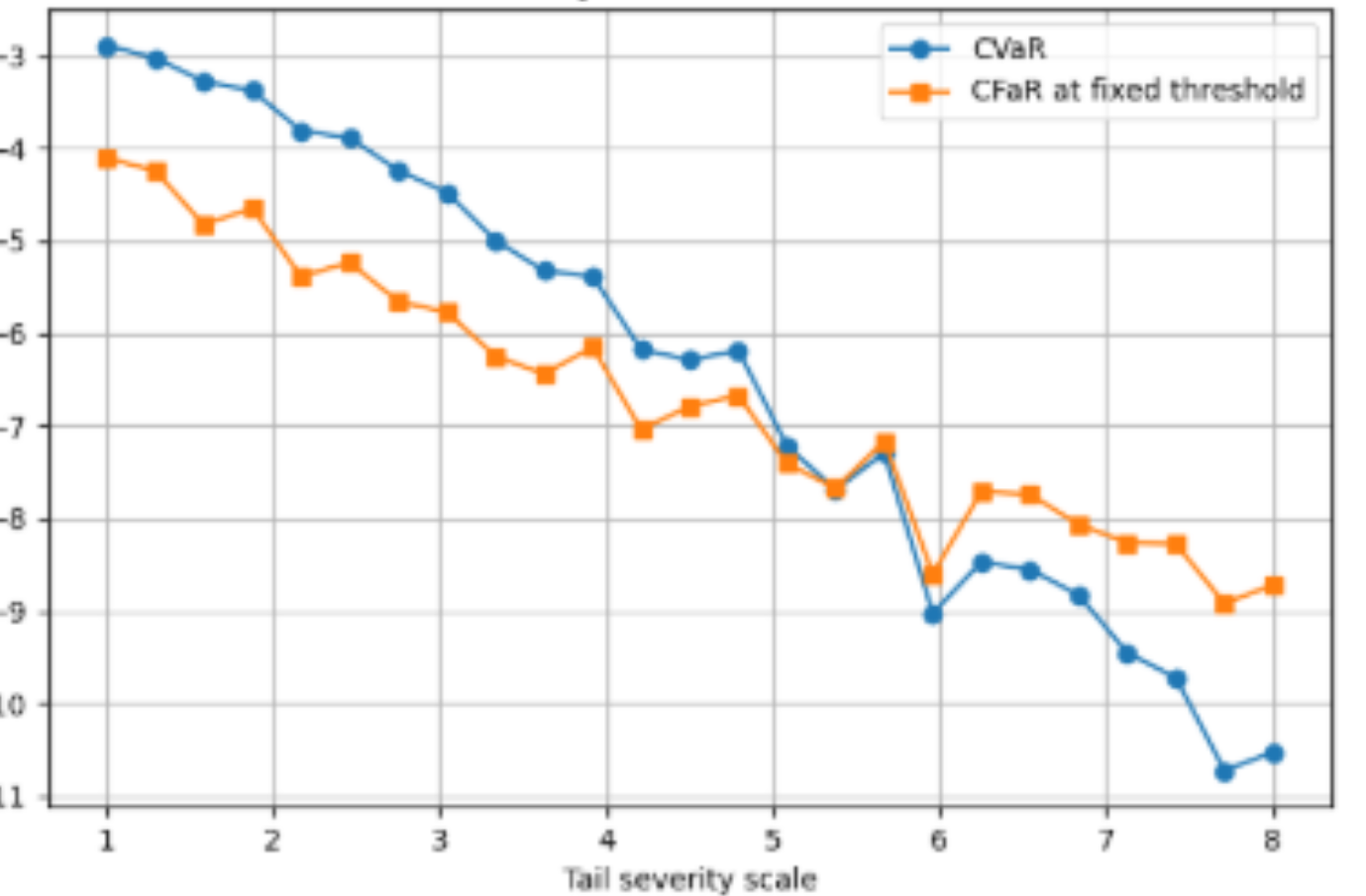
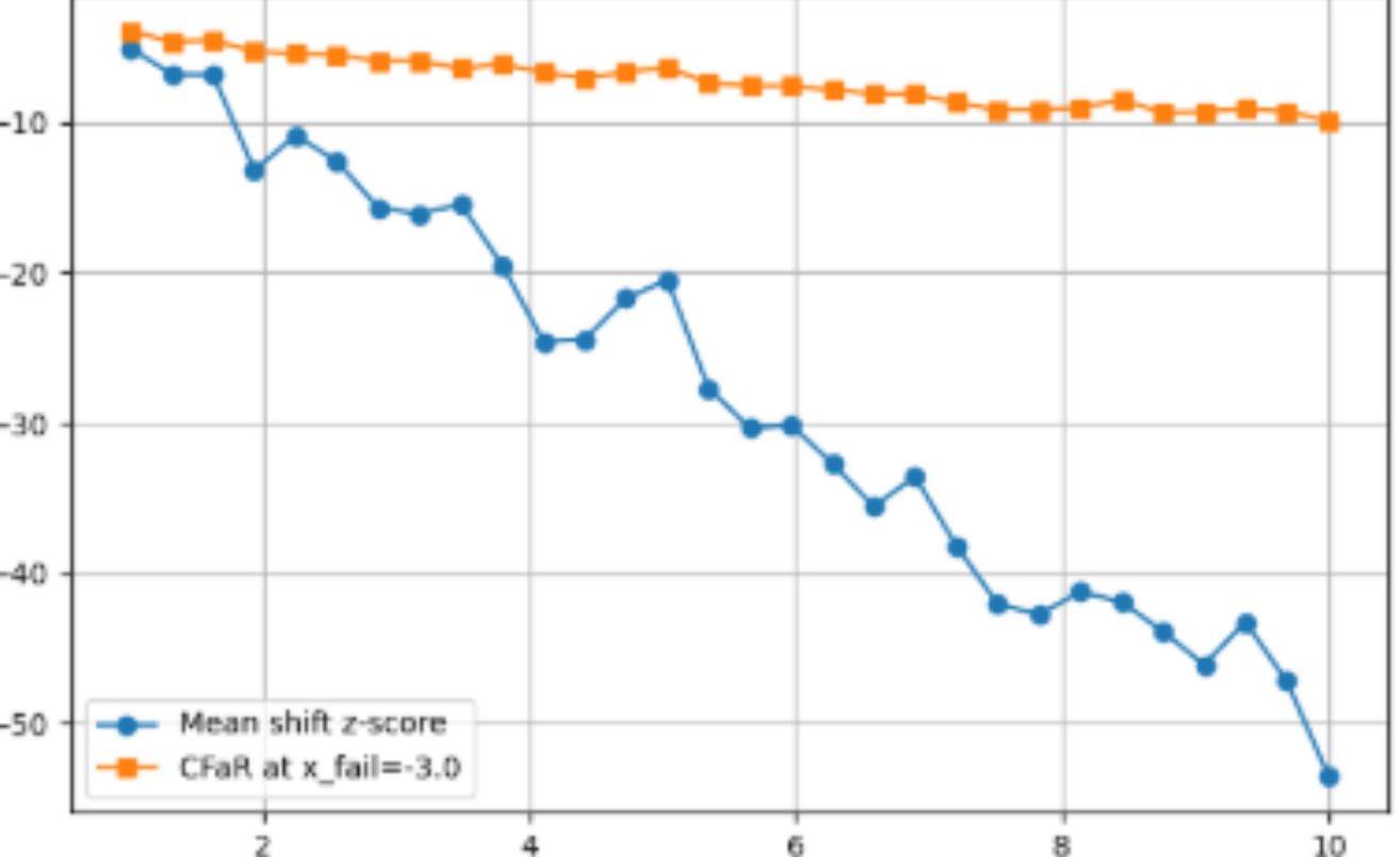
The negative impact of events occurring at the tail get predictably worse as the tail severity (degree of asymmetry) increases. Plotting the z-score of the mean as we make the tail severity larger shows only a slow and modest decrease, while the CVaR/CFaR falls precipitously. The mean does not reflect how bad a failure is, even though it tracks somewhat the probability of a failure. It’s known that humans are especially poor at judging the likelihood of long-tail events, but I suspect we are also bad at judging the impact of such events since they are even more remote to our intuition.

There are some important aspects to this model and long-tail distributions in general that are worth mentioning, because they impact how events are sampled. First, risks/failures here are not IID, despite the frequentist appearance of the distribution. The risks are better modeled dynamically (see below), since they represent time-dependent events/behaviors and critically have (and often do) have feed-forward components.

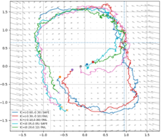
Here we can see that “events” which we modeled as p are much better represented as phases, and moving into the risk/failure phase is what the event p tried to capture. On the way to the risk phase we are not surprised to find feed-forward drivers. But once we have transitioned to the risk phase, we should also not be surprised to find stabilizing or feedback mechanisms. Some oversimplified but illustrative examples would be a planet that can no longer support humanity “recovering” in a sense to a pre-industrial state; or an overweight person spiraling toward diabetes, but then stabilized (maybe out of need) by medicine and unavoidable lifestyle changes.

Using a dynamic model instead of a frequentist approach has the benefit of making changes and impacts more local. We can see how small changes can lead to accelerated decline into a failure phase. (Sometimes we use small changes as an indication of chaotic behavior, but here we just mean “nudges” toward the risk/failure mode.) Instead of concerning ourselves only with the probability of an event y conditioned on an action x, we can see how an action brings us closer to the event region, boundary, or phase. It’s not that P(y|x) is greater than some other action, it’s that the distance (or time) between a state in which we have taken some action and the failure state is smaller: D(P(y|x),P(y)). Setting aside the complications of distances between distributions - here we mean distance on some phase portrait manifold, not in true probability space.

I think re-framing the probability of long-tail risks/events as dynamic models that show the relative distance to such events is more productive and intuitive than the pure frequentist approach. Humans are bad at asymmetric probability — and even worse when the risks are outsized and negative. Rather than thinking in terms of increasing the probability of a failure event, we should think in terms of the event boundary or region coming closer.