Modeling obscured orbital volume

When trying to view space from space, the earth blocks a cone-like volume and casts a sightline “shadow” behind it. I’m interested in exploring the amount of occluded space for an observer/satellite as a function of altitude. Given Earth’s radius R and the viewing altitude h , the observer is at position r_s, defined as angular ECEF coordinates

u_hat=[sin(theta) cos(phi), sin(theta) sin(phi), cos(theta)]
r_s=[0,0, ||r_s||]
r_hat=[0,0,1]

The angle between the observer r_hat and the “look vector” u_hat (both normalized) is m=u_hat . v_hat, where mu=1 if pointing directly away from the earth, mu=-1 if looking at the earth’s center, and mu=0 if looking exactly orthogonal.

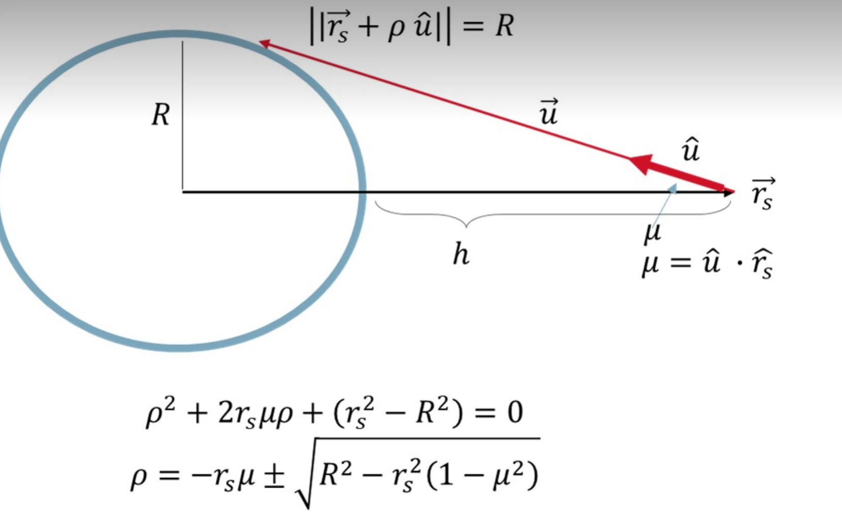
Given the distance r_s=R+h to the earth’s center, the ray that intersects with the earth is given by

|| r_s + rho u_hat ||^2 = R^2

Here, p is the range. The intersecting earth radius along the ray u is ||r_s + mu u_hat || = R which can be squared and simplified to

rho^2 + 2 r_s mu rho + (r_s^2 - R^2)=0

r_s above is the scalar given by the dot product of r_s with itself. The resulting quadratic above can be solved by WolframAlpha or Claude and results in the solutions rho=—r_s mu +/- sqrt[R^2 - r_s^2 (1-mu^2)]

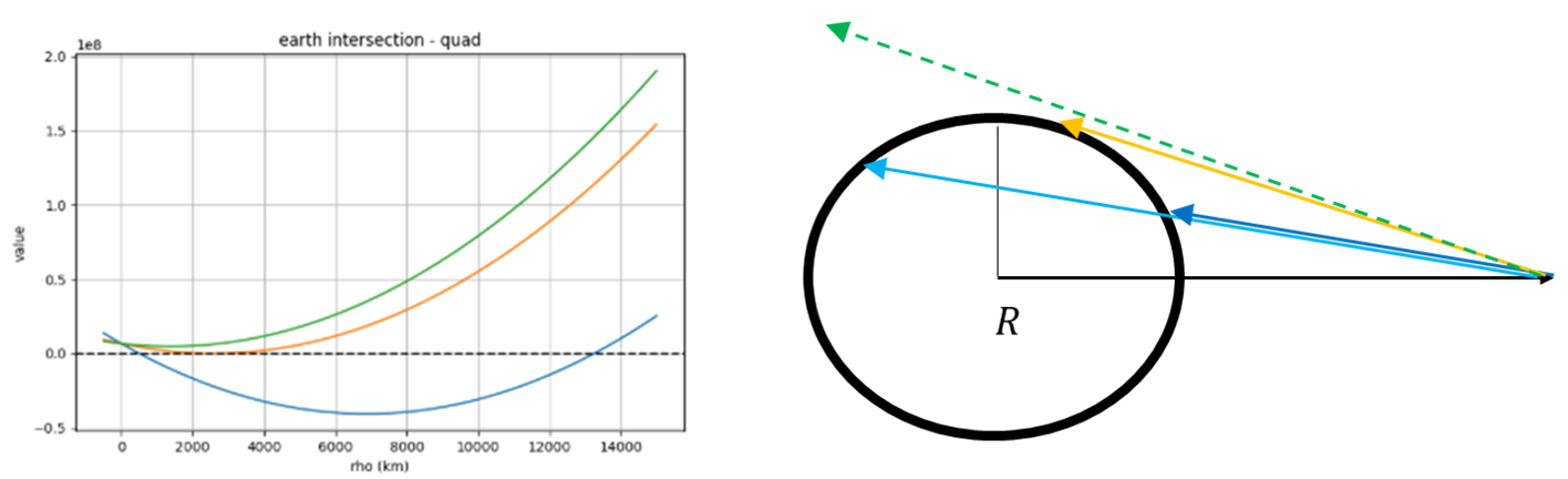
When we do this we can have 2, 1, or 0 zeroes – corresponding to intersecting with earth twice (once at near end and once at far end), once (glancing, tangent), or missing the earth entirely.

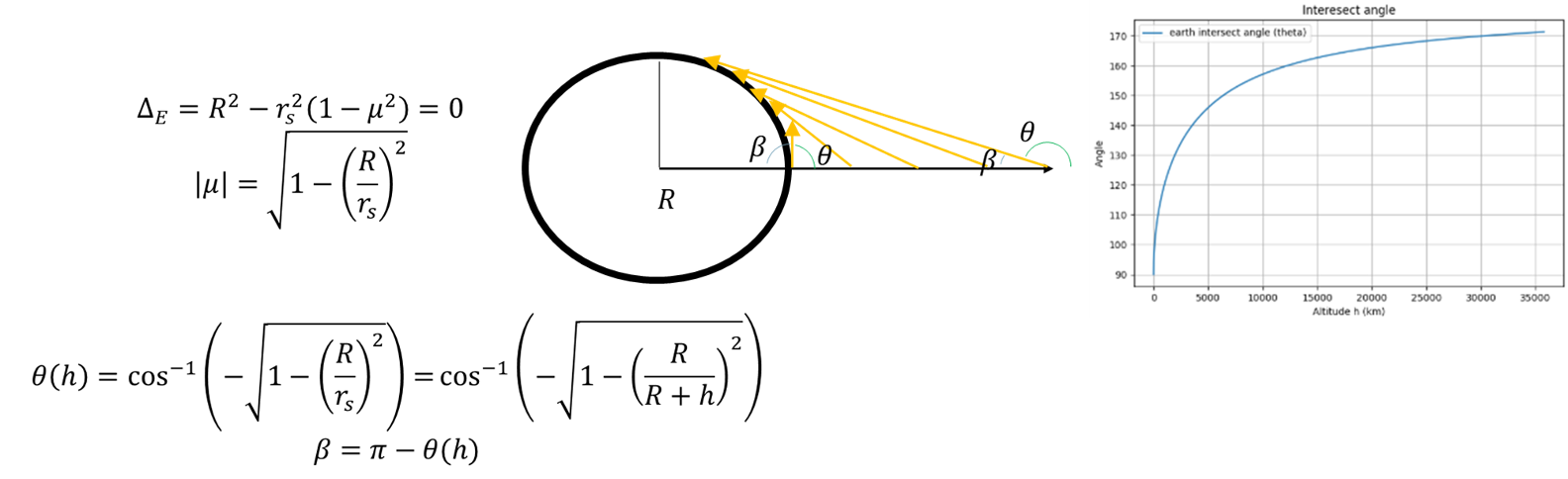
The determining element is D_E=R^2 - r_s^2 (1 - mu^2) under the radical. Earth is intersected if D_E >=0 and -r_s mu sqrt(D_E) >= 0. But we only care about D_E==0, the tangent earth intersection. For intuition, I plotted the earth intersection angle as a function of altitude, which is pretty intuitive (note theta is in the r_s ECEF frame, so it starts at 90 deg for h=0 and then gets larger; I include beta=180-theta as well, which would be the angle looking towards the earth).

Since I’m interested in finding the volume of an orbital, I just need to move the intersect equation from earth’s radius R to R’ for some orbital shell thickness. We’ll do this twice, once at a=r_1=R for the inner shell (taken to be earth’s surface in the limit for now) and a=r_2 for the outer shell.

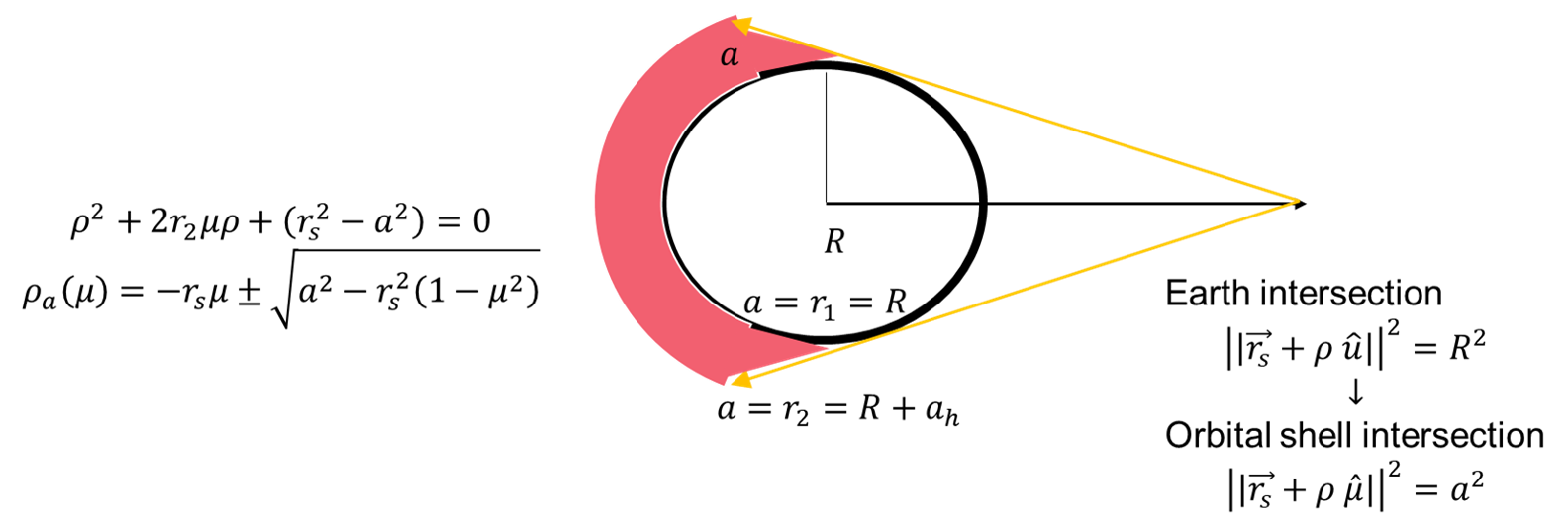
We’re working up to an equation where we can the difference between the volume of a simple spherical shell and the volume occluded by the earth for a given altitude — as a function of mu the dot product between the observer altitude and look vector when the look vector intersects the shell(s). We’ll define our spherical coordinates in the reference of the observer again, so (rho, theta, phi) where rho is the distance from the observer and theta/phi are the elevation/azimuth. For integrating we’ll define d Omega = sin(theta) d theta d phi to simplify the integral. Note this is only angular does not contain a thickness (rho) component yet, we need d rho too. rho is squared since area increases with the square as a function of distance.

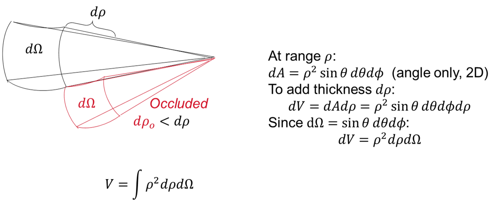
With this understanding, we can determine which directions d Omega are blocked and the ranges in those directions that are occluded d rho.

Given look angles u there are two distinct sets: I_shell(u) - the set of look angle (and length) ranges inside the shell between r_1 and r_2 - and I_occ(u): the set of ranges occluded by the earth.

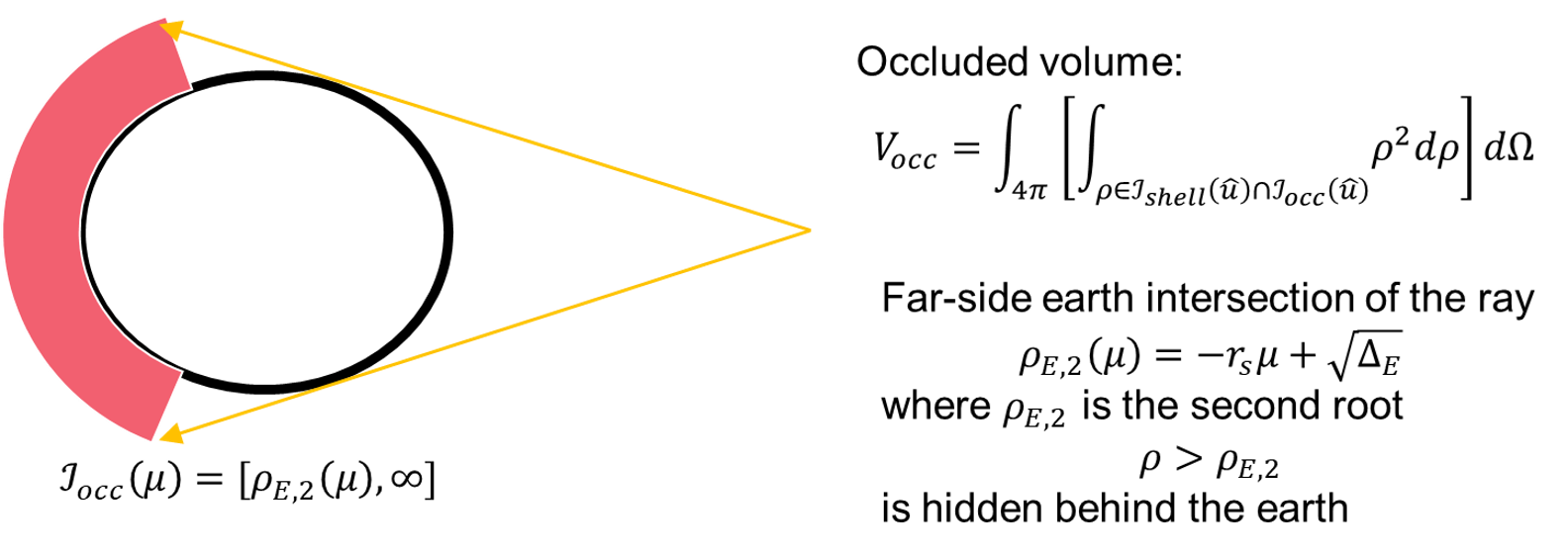
The exact volume of the occluded portion can be defined with respect to the orbital shell as rho passes from the inside of the shell to the outside, corresponding to r_1 (or r_1=rho_E,2=R ) and r_2. We still integrate with respect to rho inside. But now we can define the bounds more precisely and simply if we parameterize rho as a function of mu=[-1,1], corresponding to the pointing angle of the observer as defined above.

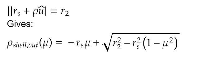
Importantly, this allows us to distinguish the 3 key intersections that the ray x(rho)=r_s + rho u_hat makes with the earth and orbitals: (1) rho_E1 and (2) rho_E2 for the first and second earth intersections, where rho_E1 < rho_E2, and (3) rho_shell,out(mu) where the ray leaves the outer shell. Solving for ||r_s + rho u_hat|| = r_2 gives us the distance rho for this intersection. So we integrate from max([rho_shell,in,rho_E2]) to rho_shell,out. In general, we will simply set the lower bound to rho_E2 to make the calculations easier. One advantage of this, practically, is it provides awareness of the lower atmosphere for air vehicles in addition to VLEO, LEO, and up.

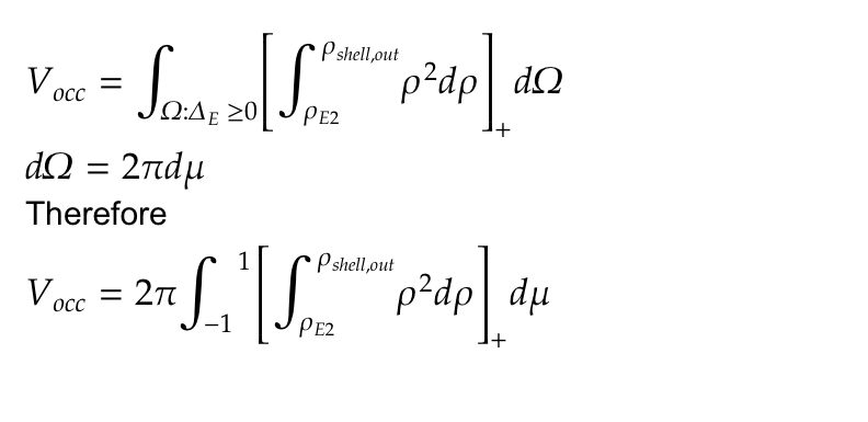
And the final occluded volume is given by first solving the inner integral:

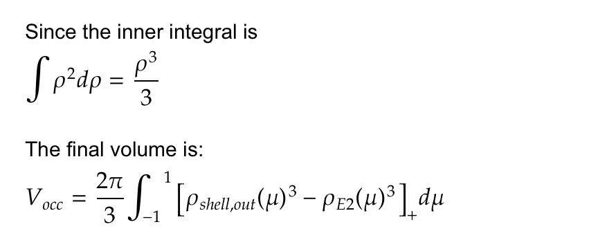
In all of these cases we have assumed the inner orbital shell is the same as the earth’s surface, more specifically the second time the observe ray intersects the earth’s surface. Parameterizing with mu and rho provided a much more convenient way to compute this volume in terms of the ray direction and ray length, respectively. The challenge came from generating the geometric interpretation and determining the intersections for rho.

We have the occluded portion defined in terms of rho and mu, but we want to compare it to the total volume of the orbital in terms of r_1=R and r_2:

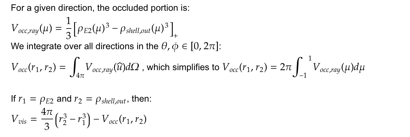
Since we have equations relating mu to altitude h by r_s=R+h, and r_s(vector)=[0,0,R+h] we can calculate the occluded and visible portions as a function of altitude:

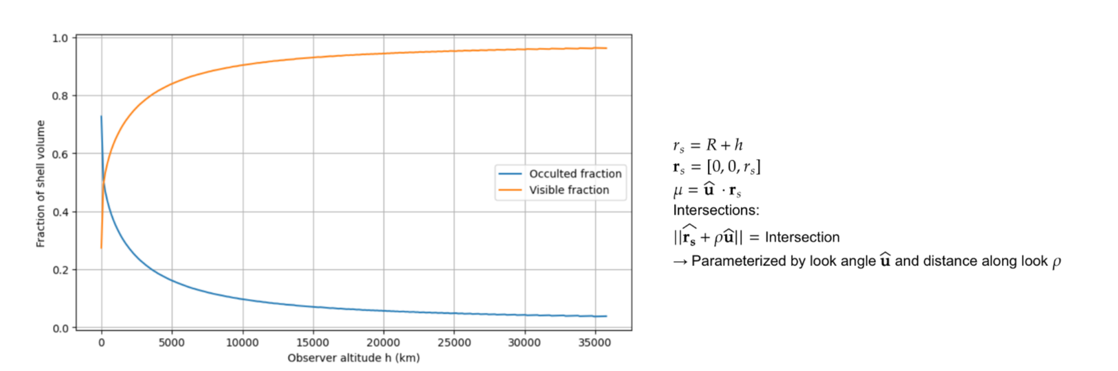
This is the result I’ve been working to.